Harmonic Potential Energy

Harmonic Oscillator

Consider a two-particle system moving in 1D. Let $r_1$ and $r_2$ be the instantaneous positions of the two particles, and let $r_1^0$ and $r_2^0$ be their equilibrium positions. On this page, we define:

• $\Delta r=r_2-r_1$ is the instantaneous distance between the two particles
• $\Delta r^0=r_2^0-r_1^0$ is the equilibrium distance between the two particles
• $\Delta r - \Delta r^0$ is the displacement from equilibrium

If the particles are displaced only slightly from $\Delta r^0$, the interaction tends to pull the system back toward equilibrium. This kind of back-and-forth motion is called harmonic motion, and the corresponding model is the harmonic oscillator.

A two-particle system is in equilibrium when the net force on the relative coordinate vanishes. For a conservative force,

so at the equilibrium position $\Delta r = \Delta r^0$ we must have

This tells us that the potential energy curve is locally flat at equilibrium. In addition, the force depends only on the derivative of $V(\Delta r)$, not on its absolute value. If we replace $V(\Delta r)$ by

then

Therefore, adding a constant does not change the physics. For this reason, we are free to choose the zero of potential energy conveniently, so we set $V(\Delta r^0)=0$.

In general, we do not know the exact form of the potential energy $V(\Delta r)$. However, if we are interested only in small displacements from equilibrium, then we can describe the potential relative to $V(\Delta r^0)=0$ by expanding it in a Maclaurin-Taylor series around the equilibrium distance:

where the primes denote differentiation with respect to $\Delta r$. Since we chose $V(\Delta r^0)=0$ and also know that $V’(\Delta r^0)=0$, the first two terms vanish. Thus, near the equilibrium distance $\Delta r^0$, we may write

where $k=V’’(\Delta r^0)$ is the curvature of the potential energy at the equilibrium distance, or the spring constant. If we choose the coordinate origin so that the equilibrium distance is at zero, that is, $\Delta r^0=0$, then the harmonic approximation simplifies to

In this shifted coordinate system, the displacement from equilibrium is simply $\Delta r$ itself, and the corresponding force becomes

This is the standard form of Hooke’s law: the force is proportional to the displacement and points in the opposite direction.

Reference: Tom W. B. Kibble and Frank H. Berkshire, Classical Mechanics, Chapter 2: Linear Motion, Sections 2.1 and 2.2.

At Temperature $T$: What Is the Size of the Fluctuation?

Define the displacement from equilibrium as $x=\Delta r - \Delta r^0$. Then the harmonic approximation gives $V(x) = \frac{1}{2}kx^2$, and the Boltzmann distribution gives $P(x) = \frac{1}{Z} \exp\left(-\frac{V(x)}{k_B T}\right)$, where the partition function is $Z = \int_{-\infty}^{\infty} \exp\left(-\frac{kx^2}{2k_B T}\right)\,dx$ and $k_B$ is the Boltzmann constant.

The ensemble average of the fluctuation is

At equilibrium, we have $\langle \Delta r \rangle = \Delta r^0$. To measure the size of the fluctuation, we therefore consider the mean-square fluctuation (MSF):

where $a = \frac{k}{2k_B T}$. Using the Gaussian integral result (ref), $\int_{-\infty}^{\infty} x^2 e^{-ax^2} dx = \frac{1}{2a}\sqrt{\frac{\pi}{a}}$, we have

What is $Z$? The partition function is $Z = \int_{-\infty}^{\infty} e^{-ax^2} dx = \sqrt{\frac{\pi}{a}}$. Therefore,

This is an important result. It tells us that:

• MSF increases with temperature
• MSF decreases when the spring constant becomes larger

Solution of Harmonic Motion

To solve the motion, combine Newton’s second law with the harmonic restoring force:

We may view this equation as a linear differential equation of the general form

where $a_2(t)=m$, $a_1(t)=0$, $a_0(t)=k$, and $b(t)=0$. Therefore, the equation of motion for $\Delta r(t)$ is a second-order linear differential equation. In operator form, we may define the linear differential operator

so that the equation of motion can be written compactly as

We now want to find a function $\Delta r(t)$ that is annihilated by this operator, that is, a function satisfying the differential equation above. For linear equations with constant coefficients, a standard approach is to try an exponential solution, because exponentials remain proportional to themselves when differentiated. We therefore assume a trial solution of the form

where $\lambda$ is a constant to be determined. Substituting this trial form into the equation of motion gives

Since $e^{\lambda t}$ is never zero, we can divide both sides by it and obtain

Thus there are two linearly independent exponential solutions $e^{i\omega t}$ and $e^{-i\omega t}$.

Because the differential equation is linear, any linear combination of these solutions is also a solution. Therefore,

where $A$ and $B$ are arbitrary complex numbers. Although this expression is written in terms of complex exponentials, the physical displacement must be real. Using Euler’s formula,

we can rewrite the general real-valued solution in the equivalent form

where $a$ and $b$ are real constants determined by the initial conditions. This shows that the motion is sinusoidal, with angular frequency $\omega=\sqrt{\frac{k}{m}}$; equivalently, $k=m\omega^2$, so the spring constant is proportional to the frequency squared.

How can we determine the constants $a$ and $b$ from the initial position and initial velocity?

This is the standard 1D solution for harmonic motion. It tells us that the particle oscillates with angular frequency

Figure source: Simple English Wikipedia: Angular frequency

In general physics, angular frequency $\omega$ measures how fast a system moves through an angle or phase. For an object rotating around a circle, it is defined by $\omega = \frac{d\theta}{dt}$, where $\theta$ is the angle swept out in time $t$. So a larger $\omega$ means the system moves through its cycle more quickly.

In the figure, the rotating radius sweeps out an angle $\theta$. As time passes, the angle changes continuously, and $\omega$ tells us how rapidly that change happens. This is why angular frequency is commonly associated with rotation.

For our two-particle motion in 1D, the particles do not literally move in a circle. However, the solution

still contains the phase $\omega t$. That phase plays the same mathematical role as an angle in circular motion. So even though the motion is back-and-forth along one line, $\omega$ still measures how fast the oscillation goes through one cycle.

Harmonic Motion in 2D

Now we extend the same idea to 2D. In this section, we define:

• $\mathbf{r}_1 = [x_1\ y_1]^T$ and $\mathbf{r}_2 = [x_2\ y_2]^T$ are the position vectors.
• $\mathbf{r}_1^0 = [x_1^0\ y_1^0]^T$ and $\mathbf{r}_2^0 = [x_2^0\ y_2^0]^T$ are the equilibrium position vectors.
• $\Delta \mathbf{r} = \mathbf{r}_2 - \mathbf{r}_1$ is the instantaneous separation vector.
• $\Delta \mathbf{r}^0 = \mathbf{r}_2^0 - \mathbf{r}_1^0$ is the equilibrium separation vector.
• $\Delta \mathbf{r} - \Delta \mathbf{r}^0$ is the displacement of the separation vector from equilibrium.

Remember, lowercase regular symbols denote scalars, while boldface symbols denote vectors or matrices.

Now we know that the force acting on the system has two components, one in the $x$-direction and one in the $y$-direction:

Here, $\nabla_{\Delta \mathbf{r}} V$ is the gradient of the potential $V$ with respect to the separation vector $\Delta \mathbf{r}$, so it is the first derivative of $V$ with respect to $\Delta \mathbf{r}$. The matrix of second derivatives is the $2\times 2$ Hessian matrix:

The matrix $\mathbf{H}$ tells us how strongly the system resists displacement in each direction and whether motions in different directions are coupled. If this resistance is the same in every direction, then the motion is called isotropic; otherwise, it is anisotropic. In the isotropic case, the Hessian matrix is proportional to the identity matrix,

where $k=\dfrac{\partial^2 V}{\partial (\Delta x)^2}=\dfrac{\partial^2 V}{\partial (\Delta y)^2}$, the mixed derivative vanishes, and $\mathbf {I}$ is the identity matrix. Then the restoring force has the same strength in every direction.

Similar to Eq. 6, when the system is only slightly displaced from equilibrium, we expand $V$ using a Taylor series:

where $\mathbf{H}$ is the Hessian matrix of second derivatives of the potential evaluated at $\Delta \mathbf{r}^0$. Since $\Delta \mathbf{r}^0$ is the equilibrium separation vector, the first derivative vanishes:

If we also choose the zero of potential energy so that $V(\Delta \mathbf{r}^0)=0$, then the expansion reduces to

And again, if we choose the coordinate system so that $\Delta \mathbf{r}^0 = \mathbf{0}$, then we have

How can we calculate the force, now?

We now combine Eq. 26 with Newton’s second law. For the relative coordinate, the equation of motion becomes

Thermal Fluctuation in 2D

Let us define the displacement from equilibrium as $\mathbf{x} = \Delta \mathbf{r} - \Delta \mathbf{r}^0$. Using Eq. 24, the harmonic potential can be written as

At thermal equilibrium, the probability density of the displacement vector is given by the Boltzmann distribution:

where the partition function is $Z=\int \exp!\left(-\frac{1}{2k_B T}\mathbf{x}^T \mathbf{H} \mathbf{x}\right)\,d\mathbf{x}$. To describe the size of the fluctuation, we consider the covariance matrix

This is the 2D analogue of the 1D result $\langle x^2 \rangle = k_B T/k$. In 1D, the spring constant is the scalar $k$; in 2D, it is replaced by the Hessian matrix $\mathbf{H}$, so the fluctuation is controlled by the inverse Hessian.

The mean-square size of the fluctuation is the ensemble average of the squared magnitude:

Therefore, the root-mean-square fluctuation is

These equations show that the fluctuations are larger at higher temperature and smaller when the Hessian has larger eigenvalues, that is, when the system is stiffer. This same idea is generalized further in Gaussian network models, where fluctuation amplitudes and correlations are obtained from the inverse of a network matrix.

Solution of Harmonic Motion in 2D

To solve Eq. 27, we again try an exponential form. Since the displacement is now a vector, we assume

where $\mathbf{u}$ is a constant vector and $\lambda$ is a constant to be determined. Substituting this trial solution into Eq. 27 gives

Since $e^{\lambda t} \neq 0$, we can divide by it and obtain

Therefore, $\mathbf{u}$ must be an eigenvector of $\mathbf{H}$, and the corresponding eigenvalue is $\mu = -m \lambda^2$. Since $\mathbf{H}$ is a $2\times 2$ matrix, it has two eigenvalues, which we denote by $\mu_1$ and $\mu_2$, with corresponding eigenvectors $\mathbf{u}_1$ and $\mathbf{u}_2$.

Let us define the angular frequencies $\omega^2 = \mu / m = -\lambda^2$ ($\mu=m\omega^2$, eigenvalue is proportional to frequency square), then we obtain $\lambda = \pm i\omega_1$, $\lambda = \pm i\omega_2$. Therefore, the exponential solutions are

Using Euler’s formula, we can rewrite the general real-valued solution as

, where $a_1$, $b_1$, $a_2$, and $b_2$ are constants determined by the initial conditions.

In this form, the meaning becomes clearer. The total motion is the sum of two independent oscillations, one along the direction of $\mathbf{u}_1$ and the other along the direction of $\mathbf{u}_2$.

Each of these oscillations is called a normal mode. A normal mode is a pattern of motion in which all coordinates oscillate with the same single frequency and keep a fixed direction pattern determined by the eigenvector. In our 2D case:

• $\mathbf{u}_1$ gives the first normal mode, with frequency $\omega_1$
• $\mathbf{u}_2$ gives the second normal mode, with frequency $\omega_2$

Therefore, although the motion may look complicated in the original $x$-$y$ coordinates, it becomes simple when expressed in the basis of eigenvectors of the Hessian matrix. In that basis, the coupled 2D motion is decomposed into a superposition of two independent harmonic oscillators.

N-particle system in 3D

We now generalize the discussion from a two-particle system to an $n$-particle system in three dimensions. A convenient picture is a mass-spring network, where each particle is represented by a node and each interaction is represented by a spring.

Figure source: Wikipedia: Gaussian network model

In this model, particle $i$ has position vector $\mathbf{R}_i = \begin{pmatrix} x_i \ y_i \ z_i \end{pmatrix}$, and equilibrium position vector $\mathbf{R}_i^0 = \begin{pmatrix} x_i^0 \ y_i^0 \ z_i^0 \end{pmatrix}$. Its displacement from equilibrium is

For the whole system, the instantaneous position vectors, equilibrium position vectors, and displacement vectors are

For the whole system, we define:

• $n$ is the number of particles in the system.
• $\mathbf{R}_i$ is the instantaneous position vector of particle $i$.
• $\mathbf{R}_i^0$ is the equilibrium position vector of particle $i$.
• $\Delta \mathbf{R}_i = \mathbf{R}_i - \mathbf{R}_i^0$ is the displacement vector of particle $i$ from equilibrium.
• $\mathbf{R}_{ij} = \mathbf{R}_j - \mathbf{R}_i$ is the instantaneous separation vector between particles $i$ and $j$.
• $\mathbf{R}_{ij}^0 = \mathbf{R}_j^0 - \mathbf{R}_i^0$ is the equilibrium separation vector between particles $i$ and $j$.

The change in separation vector from equilibrium is \(\Delta \mathbf{R}_{ij}=\mathbf{R}_{ij}-\mathbf{R}_{ij}^0 = (\mathbf{R}_j - \mathbf{R}_i) - (\mathbf{R}_j^0 - \mathbf{R}_i^0) = \Delta \mathbf{R}_j - \Delta \mathbf{R}_i\)

It means that the change in separation vector is just the difference of the two particle displacement vectors. For one interacting pair $(i,j)$, the harmonic potential energy is

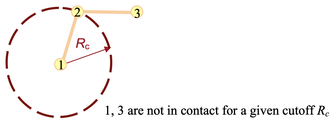
Here, $\mathbf{H}{ij}$ is the 3x3 Hessian matrix for the interaction between particles $i$ and $j$, evaluated at $\mathbf{R}{ij}^0$:

As a concrete example, consider a tri-peptide-like system with three particles, labeled $1$, $2$, and $3$, as shown below. Suppose that particles $1$ and $2$ are in contact, particles $2$ and $3$ are in contact, but particles $1$ and $3$ are not in contact for the chosen cutoff distance $R_c$.

In this case, the connectivity matrix is

Therefore, only two pair interactions contribute to the total potential:

Using Eq. 46, this becomes

Since $\mathbf{R}{ij} - \mathbf{R}{ij}^0 = \Delta \mathbf{R}_j - \Delta \mathbf{R}_i$, we may rewrite the total potential in terms of the particle displacements:

Now collect the displacements into the stacked vector

Then the same potential can be written in quadratic form,

where the tri-peptide system Hessian is the $9\times 9$ block matrix

Prove equation 48 and equation 49?

In the isotropic GNM approximation with a uniform spring constant $\gamma$, we take

Then Eq. 46h becomes

with

This is the simplest explicit example of how the full system Hessian is assembled from pair interactions and how, under the GNM approximation, it reduces to a Kirchhoff matrix times the $3\times 3$ identity.

The total harmonic potential energy of the system is obtained by summing over all connected pairs:

, where $\mathbf{H}$ is the full $3n \times 3n$ system Hessian, built from all the pair blocks $\mathbf{H}_{ij}$

Then $\mathbf{H}^{(g)}_{ij}$ is the $(i,j)$ block of this full matrix

The factor of $\frac{1}{2}$ avoids counting each pair twice.

In Gaussian network-type models, the connectivity is usually determined by a cutoff distance $r_c$: particles $i$ and $j$ are connected if

If all connected pairs are assigned the same spring constant $\gamma$, then the total potential simplifies to

This isotropic, uniform-spring approximation is the key simplification behind the Gaussian network model (GNM).

The force acting on particle $i$ is obtained from the total potential by \(\mathbf{F}_i = -\nabla_{\mathbf{R}_i} V_{\text{total}}. \tag{57}\)

Applying Newton’s second law to every particle gives a set of $n$ coupled vector equations:

Collecting all particle displacements into the stacked vector $\Delta \mathbf{R}$, the linearized equation of motion near equilibrium can be written compactly as

where $M$ is the mass matrix and $\mathbf{H}$ is now the full $3n\times 3n$ Hessian matrix of the system.

Solution of Harmonic Motion for an N-particle System in 3D

To solve Eq. 53, we again try an exponential solution, now for the full $3n$-dimensional displacement vector:

where $\mathbf{U}$ is a constant $3n$-dimensional vector.

Substituting Eq. 54 into Eq. 53 gives

Since $e^{\lambda t} \neq 0$, we obtain

This is the matrix generalization of the eigenvalue equation we saw in 2D. If all particles have the same mass $m$, then $M = mI$, and Eq. 56 becomes

Therefore, $\mathbf{U}$ must be an eigenvector of the full Hessian matrix $\mathbf{H}$, and the corresponding eigenvalue $\mu$ satisfies

If the eigenvalues of $\mathbf{H}$ are $\mu_1,\mu_2,\dots,\mu_{3n}$, then the corresponding angular frequencies are

Each eigenvector $\mathbf{U}_k$ gives one normal mode of the entire system. The general real-valued solution can therefore be written as

Here $a_k$ and $b_k$ are constants determined by the initial conditions.

This expression has exactly the same structure as the 2D two-particle case, except that the sum now runs over all $3n$ normal modes. Each mode describes a collective pattern of motion involving all particles in the system.

In practice, some of these modes correspond to rigid-body translations and rotations, which do not deform the structure and therefore have zero or near-zero frequency. The remaining nonzero-frequency modes describe the internal vibrations of the network and are the main objects of interest in elastic network models.

In the language of GNM, we usually do not follow the full time-dependent vector solution in Eq. 60. Instead, we use the isotropic network assumption to study fluctuation amplitudes and correlations from the inverse of the Kirchhoff matrix $\Gamma$. Thus, Eq. 60 is best viewed as the more detailed directional analogue, while GNM keeps the same network idea but focuses on scalar fluctuation statistics rather than explicit vector-valued motion.