Week 1: Introduction to ENMs
Topics
- Two widely known ENMs with numerous applications
- What do ENMs study?
- Each structure encodes a unique dynamics
- What do ENMs do?
- What does a spring actually do?
- What is the mean-square fluctuation of a two-particle system in a harmonic potential at temperature T?
Two widely known ENMs with numerous applications
Elastic Network Models (ENMs) is a coarse-grained model used to study structural dynamics and conformational transitions of proteins and large biomolecules.
- Gaussian network model (GNM)
- Bahar I, Atilgan AR, Erman B (1997) Direct evaluation of thermal fluctuations in protein Folding & Design 2: 173-181.
- Li H, Chang YY, Yang LW, Bahar I (2016) iGNM 2.0: the Gaussian network model database for bimolecular structural dynamics Nucleic Acids Res 44: D415-422
- Anisotropic Network model (ANM)
- Atilgan AR, Durrell SR, Jernigan RL, Demirel MC, Keskin O, Bahar I (200I) Anisotropy of fluctuation dynamics of proteins with an elastic network model Biophys J 80: 505-515.
- Eyal E, Lum G, Bahar I (2015) The Anisotropic Network Model web server at 2015 (ANM 2.0) Bioinformatics 3l: 1487-9
What do ENMs study?
- Collective (global) couplings motions (link to low frequency mode).
- Global in the sense that they involve entire structure (are not localized).
- They are important because they are the overall structure favors (they call intrinsic dynamics) - what structure is going to do during its biological activities
- Therefore, these motions are being recruited for biological functioning.
- Fluctuation of structural elements (e.g. residues, secondary structures, domains, or entire subunits) from their mean positions.
- Identifying functional sites - mechanical residues, sensors and effectors (perturbation response analysis), signaling sites (allosteric communication).
- Predicting pathogenic protein variants
ref: dynomics.pitt.edu
Each structure encodes a unique dynamics?
What do ENMs do?
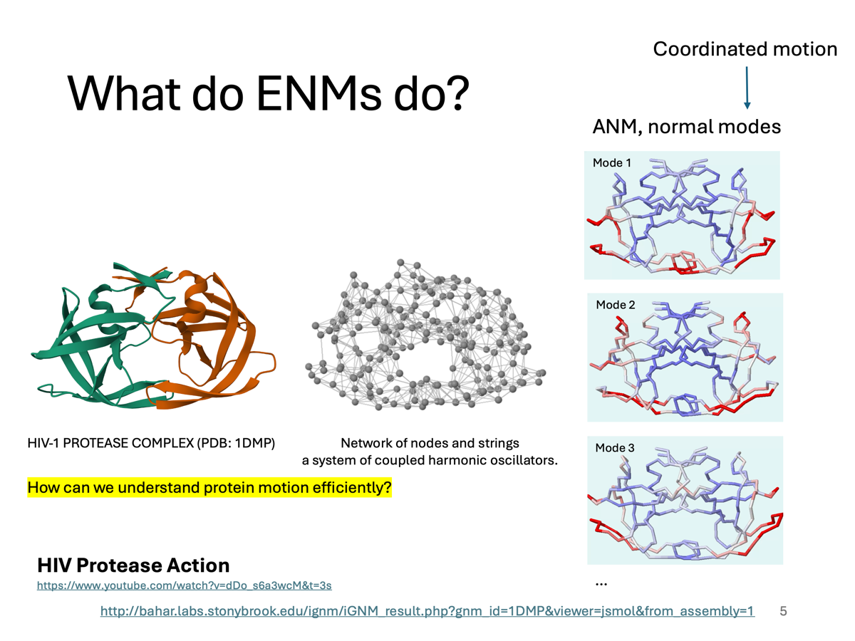
Protein is not static — it moves in order to function. For example, HIV-1 protease has flap regions that open and close to allow substrate binding. So the key question is: how can we understand protein motion efficiently?
Using ENMs, we get something called normal modes. These are the natural ways the protein prefers to move.
- Each mode represents a pattern of motion — not random movement, but coordinated motion of the entire protein.
- The first few modes — like Mode 1, 2, 3 — are the most important because they correspond to large-scale, functional motions.
- For HIV protease, these modes often correspond to flap opening and closing and breathing motions of the active site.
What does a spring actually do?
Let us define a two-particle system containing 2 particles.
Let the distance between the two particles be x, and let the interaction follow a harmonic potential:
U(x) = \frac{1}{2}kx^2
where k is the spring constant.
At temperature T, the probability distribution is given by:
P(x) = \frac{1}{Z} e^{-U(x)/(k_B T)}
where k_B is the Boltzmann constant and Z is the partition function.
The quantity we want is the mean-square fluctuation:
\langle x^2 \rangle = \int_{-\infty}^{\infty} x^2 P(x) \, dx
Substitute P(x) into the equation:
\langle x^2 \rangle
= \frac{1}{Z} \int_{-\infty}^{\infty} x^2 e^{-U(x)/(k_B T)} dx
= \frac{1}{Z} \int_{-\infty}^{\infty} x^2 e^{-kx^2/(2k_B T)} dx
Let
a = \frac{k}{2k_B T}
Then:
\langle x^2 \rangle
= \frac{1}{Z} \int_{-\infty}^{\infty} x^2 e^{-ax^2} dx
Using the Gaussian integral result (ref):
\int_{-\infty}^{\infty} x^2 e^{-ax^2} dx = \frac{1}{2a}\sqrt{\frac{\pi}{a}}
So,
\langle x^2 \rangle = \frac{1}{Z} \cdot \frac{1}{2a}\sqrt{\frac{\pi}{a}}
Now, what is Z?
The partition function is:
Z = \int_{-\infty}^{\infty} e^{-ax^2} dx = \sqrt{\frac{\pi}{a}}
Therefore,
\langle x^2 \rangle
= \frac{1}{\sqrt{\pi/a}} \cdot \frac{1}{2a}\sqrt{\frac{\pi}{a}}
= \frac{1}{2a}
Substitute back a = k/(2k_B T):
\langle x^2 \rangle = \frac{k_B T}{k}
This is an important result. It tells us that:
- the mean-square fluctuation increases with temperature
- the mean-square fluctuation decreases when the spring constant becomes larger
So a softer spring gives larger fluctuations, while a stiffer spring gives smaller fluctuations. This is the physical idea behind why ENMs can connect network stiffness to molecular fluctuations.
How do we extend this to 2D?
In the previous example, the fluctuation x was only along one direction.
Now let us keep the same two-particle system, but allow the relative displacement to move in two dimensions.
Let the equilibrium relative position between particle 1 and particle 2 be:
\mathbf{r}^{0} = \mathbf{r}^{0}_{1} - \mathbf{r}^{0}_{2} =
\begin{pmatrix}
x_0 \\
y_0
\end{pmatrix}
Let the instantaneous relative position be:
\mathbf{r} = \mathbf{r}_1 - \mathbf{r}_2 =
\begin{pmatrix}
x \\
y
\end{pmatrix}
Then the fluctuation vector is defined as:
\Delta \mathbf{r} = \mathbf{r} - \mathbf{r}^{0}
= \begin{pmatrix}
x \\
y
\end{pmatrix}
-
\begin{pmatrix}
x_0 \\
y_0
\end{pmatrix}
=
\begin{pmatrix}
\Delta x \\
\Delta y
\end{pmatrix}
If the interaction is isotropic, the harmonic potential is written in terms of the fluctuation from equilibrium:
U(\Delta x, \Delta y) = \frac{1}{2}k(\Delta x^2 + \Delta y^2)
This can also be written in matrix form:
U(\Delta \mathbf{r}) = \frac{1}{2} \Delta \mathbf{r}^T
\begin{pmatrix}
k & 0 \\
0 & k
\end{pmatrix}
\Delta \mathbf{r}
At temperature T, the probability distribution is:
P(\Delta x, \Delta y) = \frac{1}{Z} e^{-U(\Delta x,\Delta y)/(k_B T)}
= \frac{1}{Z} e^{-k(\Delta x^2+\Delta y^2)/(2k_B T)}
Now the fluctuation is no longer described by one scalar quantity. Instead, we use the fluctuation matrix:
\langle \Delta \mathbf{r}\, \Delta \mathbf{r}^T \rangle =
\begin{pmatrix}
\langle \Delta x^2 \rangle & \langle \Delta x \, \Delta y \rangle \\
\langle \Delta y \, \Delta x \rangle & \langle \Delta y^2 \rangle
\end{pmatrix}
Because the spring is isotropic and the x and y directions are independent,
\langle \Delta x^2 \rangle = \frac{k_B T}{k}
\langle \Delta y^2 \rangle = \frac{k_B T}{k}
\langle \Delta x \, \Delta y \rangle = 0
Therefore,
\langle \Delta \mathbf{r}\, \Delta \mathbf{r}^T \rangle =
\frac{k_B T}{k}
\begin{pmatrix}
1 & 0 \\
0 & 1
\end{pmatrix}
If we only want the total mean-square fluctuation in 2D, then:
\langle |\Delta \mathbf{r}|^2 \rangle = \langle \Delta x^2 + \Delta y^2 \rangle
= \langle \Delta x^2 \rangle + \langle \Delta y^2 \rangle
= \frac{2k_B T}{k}
So compared with the 1D case:
- in 1D, the fluctuation is a scalar:
\langle x^2 \rangle - in 2D, the fluctuation becomes a matrix:
\langle \Delta \mathbf{r}\, \Delta \mathbf{r}^T \rangle - the total fluctuation is the sum of the contributions from each direction
This is the key step toward ENMs, where fluctuations are described in multiple dimensions and are represented by matrices rather than a single number.
What about 3D?
In 3D, the same idea still applies. The total mean-square displacement is:
\langle r^2 \rangle = \langle x^2 + y^2 + z^2 \rangle
= \langle x^2 \rangle + \langle y^2 \rangle + \langle z^2 \rangle
= \frac{3k_B T}{k}
because each Cartesian direction contributes equally:
\langle x^2 \rangle = \langle y^2 \rangle = \langle z^2 \rangle = \frac{k_B T}{k}
So the pattern is:
- in 1D:
\langle x^2 \rangle = k_B T / k - in 2D:
\langle r^2 \rangle = 2k_B T / k - in 3D:
\langle r^2 \rangle = 3k_B T / k
This is why, in ENMs, fluctuations are naturally described in 3D Cartesian space.
Now move to a 3-particle system in 3D
Now we take the next step toward ENMs. Instead of two particles, we consider three particles in 3D space. Each particle has three displacement components, so the full displacement vector becomes:
\Delta \mathbf{R} =
\begin{pmatrix}
\Delta x_1 \\
\Delta y_1 \\
\Delta z_1 \\
\Delta x_2 \\
\Delta y_2 \\
\Delta z_2 \\
\Delta x_3 \\
\Delta y_3 \\
\Delta z_3
\end{pmatrix}
So this system is described by a 9 \times 1 displacement vector.
If particles 1-2 and 2-3 are connected by harmonic springs, then the potential energy is the sum of the spring terms:
U = \frac{1}{2}k_{12} \left| \Delta \mathbf{r}_2 - \Delta \mathbf{r}_1 \right|^2
+ \frac{1}{2}k_{23} \left| \Delta \mathbf{r}_3 - \Delta \mathbf{r}_2 \right|^2
where each particle displacement is a 3D vector:
\Delta \mathbf{r}_i =
\begin{pmatrix}
\Delta x_i \\
\Delta y_i \\
\Delta z_i
\end{pmatrix}
If all spring constants are the same, so that k_{12} = k_{23} = k, then:
U = \frac{1}{2}k \left| \Delta \mathbf{r}_2 - \Delta \mathbf{r}_1 \right|^2
+ \frac{1}{2}k \left| \Delta \mathbf{r}_3 - \Delta \mathbf{r}_2 \right|^2
This can be written in matrix form as:
U = \frac{1}{2} \Delta \mathbf{R}^T H \Delta \mathbf{R}
where H is now a 9 \times 9 Hessian matrix.
This is the direct extension of the earlier cases:
- 1D, 2 particles: one scalar spring coordinate
- 2D, 2 particles: one 2D fluctuation vector
- 3D, 2 particles: one 3D fluctuation vector
- 3D, 3 particles: one multi-particle displacement vector and a Hessian matrix
Then the fluctuation relation becomes:
\langle \Delta \mathbf{R} \Delta \mathbf{R}^T \rangle = k_B T \, H^{-1}
More precisely, because rigid-body motions make H singular, in practice we use the pseudoinverse:
\langle \Delta \mathbf{R} \Delta \mathbf{R}^T \rangle = k_B T \, H^{\dagger}
This is exactly the ENM idea:
- build the network of connected particles
- write the harmonic potential
- construct the Hessian matrix
- use its inverse or pseudoinverse to obtain fluctuations and correlations
A very useful interpretation is:
- the diagonal blocks describe how much each particle fluctuates
- the off-diagonal blocks describe how motions of different particles are correlated
For example,
\langle \Delta \mathbf{r}_1 \Delta \mathbf{r}_2^T \rangle
tells us how particle 1 and particle 2 move together.
So for a 3-particle system in 3D, the main result is no longer just one number like \langle x^2 \rangle.
The main result is a fluctuation matrix:
\langle \Delta \mathbf{R} \Delta \mathbf{R}^T \rangle
This is the real doorway into Gaussian Network Model and Anisotropic Network Model.